Machine Learning
Machine Learning
Course: Stanford / Coursera — Andrew Ng Week: 1–11 | Started: July 1, 2019
Table of Contents
- What is Machine Learning?
- Types of Learning
- Model Representation
- Cost Function
- Gradient Descent
- Multivariate Linear Regression
- Feature Scaling
- Normal Equation
- Logistic Regression
- Multiclass Classification
- Regularization
- Neural Networks
- ML Diagnostics
- Designing ML Systems
- Support Vector Machines
- K-Means Clustering
- Dimensionality Reduction & PCA
- Anomaly Detection
- Recommender Systems
- Large-Scale Machine Learning
- Application Example: Photo OCR
What is Machine Learning?
“Machine learning is a science of getting computers to learn without being explicitly programmed.” — Arthur Samuel (popularized by Andrew Ng)
Formal definition (Tom Mitchell): A computer program is said to learn from experience E with respect to some task T and some performance measure P, if its performance on T, as measured by P, improves with experience E.
Example — Playing Checkers
| Symbol | Definition |
|---|---|
| E | Experience of playing many games of checkers |
| T | The task of playing checkers |
| P | Probability that the program wins the next game |
Types of Learning
Supervised Learning
The algorithm is given a labeled dataset — every training example has a known “right answer.” The goal is to learn a mapping from inputs to outputs.
Key characteristics:
- Labeled training data with direct feedback
- Goal: predict output for unseen inputs
Two main problem types:
| Type | Output | Example |
|---|---|---|
| Regression | Continuous value | Predicting house prices |
| Classification | Discrete category | Tumor: benign (0) or malignant (1) |
Note: Classification can have more than 2 categories — e.g., 0 = benign, 1 = malignant type A, 2 = malignant type B.
Unsupervised Learning
The algorithm is given data with no labels. It must find hidden structure on its own — we don’t tell it what the “right answer” looks like.
Key characteristics:
- No labeled examples, no feedback
- Approach problems with little or no idea what results should look like
Two main techniques:
| Technique | Description | Example |
|---|---|---|
| Clustering | Automatically groups data into bands of similar or related items | Group users by lifespan, roles, location |
| Non-clustering | Find structure in a chaotic environment | Cocktail party problem — separating voices from mixed audio |
Reinforcement Learning (mentioned briefly): the algorithm learns by interacting with an environment and receiving rewards or penalties — covered separately.
Model Representation
Linear regression draws the best-fit straight line through data in a scatter plot. This line is called the regression line and is useful for making predictions.
Training Set — Housing Prices Example
| Size in ft² (x) | Price in $1000s (y) |
|---|---|
| 2104 | 460 |
| 1416 | 232 |
| 1534 | 315 |
| 852 | 178 |
| … | … |
Notation
| Symbol | Meaning |
|---|---|
| m | Number of training examples |
| x | Input variable / feature |
| y | Output variable / target variable |
| (x, y) | Single training example |
| (x⁽ⁱ⁾, y⁽ⁱ⁾) | The i-th training example (i-th row in the table) |
How the Supervised Learning Pipeline Works
Training Set
     │
     ▼
Learning Algorithm
     │
     ▼
  h (hypothesis)
     │
  x ──► h(x) ──► ŷ (predicted output)
The hypothesis h maps input x to a predicted output ŷ.
Hypothesis Function — Univariate Linear Regression
For a single input feature, the hypothesis is:
\[h_\theta(x) = \theta_0 + \theta_1 x\]- θ₀ — the y-intercept (bias term)
- θ₁ — the slope (weight for feature x)
This is called univariate linear regression — one variable, one feature.
Cost Function
The cost function measures how wrong the hypothesis is across all training examples. We want to choose θ₀ and θ₁ to minimize it.
Goal: Choose θ₀, θ₁ so that h(x) is as close to y as possible for all training examples (x, y).
Mean Squared Error (MSE) Cost Function
\[J(\theta_0, \theta_1) = \frac{1}{2m} \sum_{i=1}^{m} \left( h_\theta(x^{(i)}) - y^{(i)} \right)^2\]- The ½ is a convenience factor that cancels when taking the derivative
- This is also called the squared error loss function
Optimization objective:
\[\min_{\theta_0,\, \theta_1} \; J(\theta_0, \theta_1)\]Intuition — Simplified Example (θ₀ = 0)
Set θ₀ = 0 to simplify: h(x) = θ₁x (line through the origin). Now J is purely a function of θ₁ — a parabola.
Worked example with 3 training points: (1,1), (2,2), (3,3)
| θ₁ | h(x) | J(θ₁) |
|---|---|---|
| 0 | 0 | ~1.67 |
| 0.5 | 0.5x | ~0.58 |
| 1 | x | 0 ← optimal |
At θ₁ = 0.5:
\[J(0.5) = \frac{1}{2 \times 3}\left[(0.5-1)^2 + (1-2)^2 + (1.5-3)^2\right] = \frac{1}{6}[0.25 + 1 + 2.25] \approx 0.58\]When we plot J(θ₁) vs θ₁, we get a convex parabola with a single global minimum — this is the ideal landscape for optimization.
Visualizing with Both Parameters
When θ₀ ≠ 0, plotting J(θ₀, θ₁) gives a 3D bowl-shaped surface (convex). We can also view it as 2D contour plots — the center of the smallest contour ellipse is the minimum.
Gradient Descent
Gradient descent is the algorithm used to find the values of θ₀ and θ₁ that minimize J.
Intuition: Imagine standing on a hilly landscape and taking small steps downhill in the direction of steepest descent — eventually reaching the valley (minimum).
Algorithm
Start with some initial θ₀, θ₁ (often both = 0), then repeat until convergence:
\[\theta_j := \theta_j - \alpha \frac{\partial}{\partial \theta_j} J(\theta_0, \theta_1) \quad \text{for } j = 0, 1\]Critical: Update θ₀ and θ₁ simultaneously using temp variables, not sequentially.
temp0 := θ₀ − α · ∂J/∂θ₀
temp1 := θ₁ − α · ∂J/∂θ₁
θ₀ := temp0
θ₁ := temp1
α (alpha) is the learning rate — controls the step size:
- Too small → very slow convergence
- Too large → may overshoot, fail to converge, or diverge
Gradient Descent for Linear Regression
After computing the partial derivatives of the MSE cost function:
Repeat until convergence:
\[\theta_0 := \theta_0 - \alpha \cdot \frac{1}{m} \sum_{i=1}^{m} \left(h_\theta(x^{(i)}) - y^{(i)}\right)\] \[\theta_1 := \theta_1 - \alpha \cdot \frac{1}{m} \sum_{i=1}^{m} \left(h_\theta(x^{(i)}) - y^{(i)}\right) \cdot x^{(i)}\](Update both simultaneously)
Key Properties
- “Batch” Gradient Descent — each update uses the entire training set (all m examples)
- The cost function J of linear regression is always convex (bowl-shaped) → only one global minimum, no local minima
- Starting from any initial guess and repeatedly applying these updates will make the hypothesis more and more accurate
Multivariate Linear Regression
Week 2 — extends linear regression to multiple input features (variables) to better predict the output.
Training Set — Extended Housing Example
| Size (ft²) | # Bedrooms | # Floors | Age (yrs) | Price ($1000s) |
|---|---|---|---|---|
| 2104 | 5 | 1 | 45 | 460 |
| 1416 | 3 | 2 | 40 | 232 |
| 1534 | 3 | 2 | 30 | 315 |
| 852 | 2 | 1 | 36 | 178 |
Notation
| Symbol | Meaning |
|---|---|
| n | Number of features |
| x⁽ⁱ⁾ | Input features of the i-th training example (a vector) |
| xⱼ⁽ⁱ⁾ | Value of feature j in the i-th training example |
| x₁, x₂, x₃, x₄ | Size, # bedrooms, # floors, age |
Hypothesis Function — Multivariate
\[h_\theta(x) = \theta_0 + \theta_1 x_1 + \theta_2 x_2 + \cdots + \theta_n x_n\]Vectorized form (using the convention x₀ = 1):
\[\mathbf{x} = \begin{bmatrix} x_0 \\ x_1 \\ \vdots \\ x_n \end{bmatrix} \in \mathbb{R}^{n+1}, \quad \boldsymbol{\theta} = \begin{bmatrix} \theta_0 \\ \theta_1 \\ \vdots \\ \theta_n \end{bmatrix} \in \mathbb{R}^{n+1}\] \[h_\theta(x) = \boldsymbol{\theta}^T \mathbf{x} = \theta_0 x_0 + \theta_1 x_1 + \cdots + \theta_n x_n\]Setting x₀ = 1 (a “dummy” feature) allows the entire hypothesis to be written as a clean dot product θᵀx.
Gradient Descent for Multiple Variables
Repeat until convergence (update all θⱼ simultaneously for j = 0, 1, …, n):
\[\theta_j := \theta_j - \alpha \cdot \frac{1}{m} \sum_{i=1}^{m} \left(h_\theta(x^{(i)}) - y^{(i)}\right) \cdot x_j^{(i)}\]Note that for j = 0, since x₀⁽ⁱ⁾ = 1, this reduces to the familiar θ₀ update.
Summary
| Concept | Key Idea |
|---|---|
| Supervised Learning | Learn from labeled data; predict continuous (regression) or discrete (classification) output |
| Unsupervised Learning | Find hidden structure in unlabeled data (clustering, dimensionality reduction) |
| Hypothesis h(x) | The model’s prediction function — a line (or hyperplane) for linear regression |
| Cost Function J | Measures prediction error; MSE is standard for regression |
| Gradient Descent | Iterative optimization algorithm that minimizes J by following the gradient downhill |
| Batch GD | Uses all m training examples per parameter update |
| Multivariate LR | Extends to n features using vectorized notation: h(x) = θᵀx |
Feature Scaling
To make gradient descent converge faster, get every feature into approximately the same range:
\[-1 \leq x_i \leq 1\]Without scaling, features on very different scales cause elongated contours in J — gradient descent zigzags slowly to the minimum.
Mean Normalization
Replace each feature $x_i$ with:
\[x_i \leftarrow \frac{x_i - \mu_i}{s_i}\]where $\mu_i$ is the mean and $s_i$ is the range (max − min) or standard deviation.
Example — Housing:
| Feature | Raw | Normalized |
|---|---|---|
| Size (ft²) | 2104 | $x_1 = \frac{\text{size} - 1000}{2000}$ |
| # Bedrooms | 3 | $x_2 = \frac{\text{bedrooms} - 2}{5}$ |
Learning Rate Tips
Debugging gradient descent — plot $J(\theta)$ vs. number of iterations:
- $J$ should decrease on every iteration
- If $J$ is increasing → learning rate $\alpha$ is too large (overshooting)
- If $J$ decreases very slowly → $\alpha$ too small
Choosing $\alpha$: try values like 0.001, 0.003, 0.01, 0.03, 0.1, 0.3, 1 and pick the largest one that consistently decreases $J$.
Polynomial Regression
When a straight line doesn’t fit well, combine or transform features:
- Combine features: e.g., $x_3 = x_1 \cdot x_2$ (frontage × depth = area) — still linear regression in $x_3$
- Polynomial features: $h_\theta(x) = \theta_0 + \theta_1 x + \theta_2 x^2 + \theta_3 x^3$
- Feature scaling becomes even more important here (ranges explode)
- Can also use $\sqrt{x}$ as a feature
Normal Equation
An analytical alternative to gradient descent that solves for $\theta$ directly (no iteration needed):
\[\boxed{\theta = (X^T X)^{-1} X^T y}\]Gradient Descent vs. Normal Equation
| Gradient Descent | Normal Equation | |
|---|---|---|
| Learning rate $\alpha$ | Must choose | Not needed |
| Iteration | Required | Not needed |
| Large $n$ | Works well — $O(kn^2)$ | Slow — $O(n^3)$ to compute $(X^T X)^{-1}$ |
| Threshold | Preferred when $n > 10{,}000$ | Preferred when $n \leq 10{,}000$ |
Normal Equation & Non-invertibility
Sometimes $X^T X$ is singular (non-invertible). Causes:
- Redundant/dependent features — e.g., $x_1$ = size in ft², $x_2$ = size in m² (linearly dependent)
- Too many features — $m \leq n$ (more features than training examples)
Fixes: delete redundant features, use regularization, or reduce $n$.
Use
pinv(pseudo-inverse) in Octave/MATLAB — it handles singular matrices gracefully.
Logistic Regression
Week 3 — The most widely used classification algorithm. Outputs a probability between 0 and 1.
Binary classification: $y \in {0, 1}$
- $y = 1$: positive class (presence of something, e.g., malignant tumor)
- $y = 0$: negative class (absence)
Why not linear regression? Predictions $h_\theta(x)$ can exceed 1 or go below 0, and a single outlier can skew the decision boundary badly.
Hypothesis Representation
\[h_\theta(x) = g(\theta^T x), \quad z = \theta^T x\] \[\boxed{g(z) = \frac{1}{1 + e^{-z}}} \quad \text{(Sigmoid / Logistic Function)}\]- Output: $0 \leq h_\theta(x) \leq 1$
- Interpretation: $h_\theta(x) = P(y=1 \mid x;\theta)$ — probability that $y=1$ given input $x$
- Since probabilities must sum to 1: $P(y=0 \mid x;\theta) + P(y=1 \mid x;\theta) = 1$
The sigmoid function plateaus near 0 for $z \ll 0$ and near 1 for $z \gg 0$, crossing 0.5 at $z=0$.
Decision Boundary
The decision boundary is a property of the hypothesis (i.e., $\theta$), not the training set.
Prediction rule:
\[h_\theta(x) \geq 0.5 \Rightarrow y = 1 \qquad h_\theta(x) < 0.5 \Rightarrow y = 0\]Since $g(z) \geq 0.5$ when $z \geq 0$:
\[\theta^T x \geq 0 \Rightarrow y = 1 \qquad \theta^T x < 0 \Rightarrow y = 0\]The decision boundary is the line (or surface) $\theta^T x = 0$ that separates $y=0$ and $y=1$ regions. With higher-order polynomial features, the boundary can be non-linear (circles, ellipses, etc.).
Logistic Regression Cost Function
We can’t use MSE for logistic regression — $J(\theta)$ would be non-convex with many local minima.
Per-example cost:
\[\text{Cost}(h_\theta(x), y) = \begin{cases} -\log(h_\theta(x)) & \text{if } y = 1 \\ -\log(1 - h_\theta(x)) & \text{if } y = 0 \end{cases}\]Intuition: if $y=1$ and $h_\theta(x) \to 0$, cost $\to \infty$ (penalizes confident wrong predictions heavily).
Simplified (combined) form:
\[\text{Cost}(h_\theta(x), y) = -y \log(h_\theta(x)) - (1-y)\log(1 - h_\theta(x))\]Full cost function:
\[\boxed{J(\theta) = -\frac{1}{m} \sum_{i=1}^{m} \left[ y^{(i)} \log h_\theta(x^{(i)}) + (1 - y^{(i)}) \log(1 - h_\theta(x^{(i)})) \right]}\]This is convex — gradient descent converges to the global minimum.
Gradient descent update (identical form to linear regression):
\[\theta_j := \theta_j - \alpha \frac{1}{m} \sum_{i=1}^{m} \left( h_\theta(x^{(i)}) - y^{(i)} \right) x_j^{(i)}\]Advanced Optimization
Alternatives to gradient descent that auto-select step size and are often faster:
| Algorithm | Notes |
|---|---|
| Conjugate Gradient | No need to manually pick $\alpha$, faster |
| BFGS | Quasi-Newton; faster convergence |
| L-BFGS | Memory-efficient BFGS; good for large $n$ |
These are more complex but generally outperform vanilla gradient descent. Use a library implementation — don’t write from scratch.
Multiclass Classification
One-vs-All (One-vs-Rest): for $y \in {1, 2, \ldots, K}$, train $K$ separate binary logistic regression classifiers:
\[h_\theta^{(i)}(x) = P(y = i \mid x;\theta), \quad i = 1, 2, \ldots, K\]Each classifier $h_\theta^{(i)}$ is trained to distinguish class $i$ from all other classes combined.
Prediction: given a new input $x$, pick the class with the highest probability:
\[\hat{y} = \underset{i}{\arg\max} \; h_\theta^{(i)}(x)\]Regularization
The Problem of Overfitting
| Condition | Description | Also Called |
|---|---|---|
| Underfitting | Too simple; high training error; doesn’t capture structure | High bias |
| Good fit | Generalizes well | — |
| Overfitting | Too complex; $J(\theta) \approx 0$ on training set but fails on new examples | High variance |
Overfitting occurs when we have too many features relative to training examples — the model memorizes the training data instead of learning general patterns.
Addressing overfitting:
- Reduce features — manually select, or use a model selection algorithm
- Regularization — keep all features but shrink parameter magnitudes $\theta_j$
Regularization works especially well when there are many features, each contributing a little to predicting $y$.
Regularization: Cost Function
Add a penalty term that shrinks all $\theta_j$ (except $\theta_0$, the bias):
\[\boxed{J(\theta) = \frac{1}{2m} \sum_{i=1}^{m} \left(h_\theta(x^{(i)}) - y^{(i)}\right)^2 + \frac{\lambda}{2m} \sum_{j=1}^{n} \theta_j^2}\]$\lambda$ (regularization parameter) controls the trade-off:
- Too small $\lambda$ → overfitting (no regularization effect)
- Too large $\lambda$ → underfitting (all $\theta_j \approx 0$, hypothesis becomes $h_\theta(x) \approx \theta_0$)
Small $\theta$ values → simpler hypothesis → less prone to overfitting.
Regularized Linear Regression
Gradient descent (note the shrinkage factor on $\theta_j$):
\[\theta_0 := \theta_0 - \alpha \frac{1}{m} \sum_{i=1}^{m} \left(h_\theta(x^{(i)}) - y^{(i)}\right)\] \[\theta_j := \theta_j \underbrace{\left(1 - \alpha\frac{\lambda}{m}\right)}_{\text{shrinkage}} - \alpha \frac{1}{m} \sum_{i=1}^{m} \left(h_\theta(x^{(i)}) - y^{(i)}\right) x_j^{(i)}, \quad j \geq 1\]The factor $(1 - \alpha\lambda/m) < 1$ slightly shrinks $\theta_j$ on every step.
Normal equation with regularization:
\[\theta = \left(X^T X + \lambda L\right)^{-1} X^T y\] \[L = \begin{bmatrix} 0 & & & \\ & 1 & & \\ & & \ddots & \\ & & & 1 \end{bmatrix} \in \mathbb{R}^{(n+1)\times(n+1)}\]Adding $\lambda L$ also fixes the non-invertibility issue when $m \leq n$.
Regularized Logistic Regression
\[J(\theta) = -\frac{1}{m} \sum_{i=1}^{m} \left[ y^{(i)} \log h_\theta(x^{(i)}) + (1-y^{(i)}) \log(1 - h_\theta(x^{(i)})) \right] + \frac{\lambda}{2m} \sum_{j=1}^{n} \theta_j^2\]Gradient descent updates are the same form as regularized linear regression (just with the logistic hypothesis).
Neural Networks
Motivation
Why not just use logistic regression with many features?
For non-linear classification with $n$ features, adding all quadratic terms gives $O(n^2/2)$ features — impractical. For computer vision (e.g., 100×100 pixel images), $n \approx 10{,}000$ pixels → millions of quadratic features. Neural networks learn complex non-linear hypotheses efficiently.
Origins: Algorithms that try to mimic how the brain works.
NN Model Representation
Biological analogy:
| Biology | Artificial NN |
|---|---|
| Dendrite (receives signals) | Input features $x_1, x_2, \ldots$ |
| Nucleus | Computation node |
| Axon (sends output) | Output $h_\theta(x)$ |
Artificial neuron: takes inputs, applies weights $\theta$, passes result through sigmoid activation $g(z) = \frac{1}{1+e^{-z}}$.
Network anatomy:
| Layer | Also Called | Contents |
|---|---|---|
| Layer 1 | Input layer | $x_0, x_1, \ldots, x_n$ (with $x_0 = 1$ bias unit) |
| Layers 2..L-1 | Hidden layers | $a_i^{(l)}$ — not directly observed |
| Layer L | Output layer | $h_\theta(x)$ |
Notation:
- $a_i^{(l)}$ — activation of unit $i$ in layer $l$
- $\Theta^{(l)}$ — weight matrix mapping layer $l$ to layer $l+1$
- If layer $l$ has $s_l$ units and layer $l+1$ has $s_{l+1}$ units, then $\Theta^{(l)} \in \mathbb{R}^{s_{l+1} \times (s_l + 1)}$
Example — 3 input features, 1 hidden layer (3 units), 1 output:
\[a_1^{(2)} = g\!\left(\Theta_{10}^{(1)}x_0 + \Theta_{11}^{(1)}x_1 + \Theta_{12}^{(1)}x_2 + \Theta_{13}^{(1)}x_3\right)\] \[a_2^{(2)} = g\!\left(\Theta_{20}^{(1)}x_0 + \Theta_{21}^{(1)}x_1 + \Theta_{22}^{(1)}x_2 + \Theta_{23}^{(1)}x_3\right)\] \[a_3^{(2)} = g\!\left(\Theta_{30}^{(1)}x_0 + \Theta_{31}^{(1)}x_1 + \Theta_{32}^{(1)}x_2 + \Theta_{33}^{(1)}x_3\right)\] \[h_\Theta(x) = a_1^{(3)} = g\!\left(\Theta_{10}^{(2)}a_0^{(2)} + \Theta_{11}^{(2)}a_1^{(2)} + \Theta_{12}^{(2)}a_2^{(2)} + \Theta_{13}^{(2)}a_3^{(2)}\right)\]Forward Propagation
Vectorized form: define $z^{(l)} = \Theta^{(l-1)} a^{(l-1)}$, then:
\[a^{(l)} = g(z^{(l)})\]Add bias $a_0^{(l)} = 1$ before computing the next layer.
Forward propagation = computing activations layer by layer, from input → hidden → output. The network learns its own features in the hidden layers.
Multiclass output: for $K$ classes, the output layer has $K$ units and $h_\Theta(x) \in \mathbb{R}^K$:
\[h_\Theta(x) \approx \begin{bmatrix}1\\0\\0\\0\end{bmatrix} \text{ (class 1)}, \quad \begin{bmatrix}0\\1\\0\\0\end{bmatrix} \text{ (class 2)}, \quad \ldots\]NN Cost Function
Setup:
- $L$ = total number of layers; $s_l$ = units in layer $l$ (excluding bias)
- Binary classification: $s_L = 1$, $y \in {0,1}$
- Multi-class ($K$ classes): $s_L = K$, $y \in \mathbb{R}^K$, $K \geq 3$
Generalized cost function (regularized):
\[\boxed{J(\Theta) = -\frac{1}{m}\sum_{i=1}^{m}\sum_{k=1}^{K} \left[y_k^{(i)}\log h_\Theta(x^{(i)})_k + (1-y_k^{(i)})\log(1 - h_\Theta(x^{(i)})_k)\right] + \frac{\lambda}{2m}\sum_{l=1}^{L-1}\sum_{i}\sum_{j}\left(\Theta_{ji}^{(l)}\right)^2}\]The double sum over $k$ accounts for all output nodes; the triple sum regularizes all weights (excluding bias terms).
Backpropagation
Goal: compute $\frac{\partial J}{\partial \Theta_{ij}^{(l)}}$ for all layers — needed for gradient descent (or advanced optimizers).
Key concept: $\delta_j^{(l)}$ = “error” of node $j$ in layer $l$ — how much that node’s activation contributed to the overall error.
Algorithm (for one training example):
- Set $a^{(1)} = x$ (forward propagation through all layers to get all $a^{(l)}$)
- Compute output error: $\delta^{(L)} = a^{(L)} - y$
- Propagate backwards: $\delta^{(l)} = (\Theta^{(l)})^T \delta^{(l+1)} \odot g’(z^{(l)})$ for $l = L-1, \ldots, 2$
- No $\delta^{(1)}$ — we don’t assign error to inputs
- Accumulate: $\Delta^{(l)} := \Delta^{(l)} + \delta^{(l+1)}(a^{(l)})^T$
For the full training set, run FP then BP for each example, then average:
\[\frac{\partial J}{\partial \Theta_{ij}^{(l)}} = \frac{1}{m}\Delta_{ij}^{(l)} + \frac{\lambda}{m}\Theta_{ij}^{(l)} \quad (j \neq 0)\]Gradient Checking
BP implementation is easy to get subtly wrong — it may appear to work but converge to a wrong solution. Gradient checking numerically verifies that BP is correct.
Numerical gradient approximation (two-sided difference):
\[\frac{dJ}{d\theta} \approx \frac{J(\theta + \varepsilon) - J(\theta - \varepsilon)}{2\varepsilon}\]For each parameter $\theta_j$:
\[\frac{\partial J}{\partial \theta_j} \approx \frac{J(\theta_1,\ldots,\theta_j+\varepsilon,\ldots,\theta_n) - J(\theta_1,\ldots,\theta_j-\varepsilon,\ldots,\theta_n)}{2\varepsilon}\]Check that DVec ≈ gradApprox. Use $\varepsilon \approx 10^{-4}$.
Important: Disable gradient checking before training — it is very slow. Use it only to verify BP, then turn it off.
Random Initialization
Symmetry problem: if all weights start at 0, every hidden unit in a layer computes the same function → all updates are identical → network never learns distinct features.
Solution — Symmetry breaking: initialize each $\Theta_{ij}^{(l)}$ to a random value in $[-\varepsilon, \varepsilon]$:
Theta = rand(out, in+1) * 2 * eps - eps
Putting It All Together
Architecture choices:
- Default: same number of units in each hidden layer
- More units per layer → more expressive, but higher computational cost
- More hidden layers → generally better, train all with same # units per layer
Training procedure:
| Step | Action |
|---|---|
| 1 | Randomly initialize all weights $\Theta$ |
| 2 | Forward propagation → compute $h_\Theta(x^{(i)})$ for each example |
| 3 | Compute cost $J(\Theta)$ |
| 4 | Backpropagation → compute all partial derivatives |
| 5 | Gradient checking → verify BP (disable afterwards) |
| 6 | Use gradient descent or advanced optimizer to minimize $J(\Theta)$ |
$J(\Theta)$ for neural networks is non-convex — gradient descent may find a local minimum. In practice, this usually works well enough.
ML Diagnostics
Machine Learning Diagnostic: a test you run to gain insight into what is/isn’t working with a learning algorithm, guiding what to try next.
What to try next when your model isn’t working:
| Action | Helps with |
|---|---|
| Get more training examples | High variance (overfitting) |
| Try smaller set of features | High variance |
| Try additional features | High bias (underfitting) |
| Add polynomial features | High bias |
| Decrease $\lambda$ | High bias |
| Increase $\lambda$ | High variance |
Evaluating a Hypothesis
Split data into training set and test set (typically 70/30).
Linear regression — test set error:
\[J_{\text{test}}(\theta) = \frac{1}{2m_{\text{test}}} \sum_{i=1}^{m_{\text{test}}} \left(h_\theta(x^{(i)}_{\text{test}}) - y^{(i)}_{\text{test}}\right)^2\]Logistic regression — test set error:
\[J_{\text{test}}(\theta) = -\frac{1}{m_{\text{test}}} \sum_{i=1}^{m_{\text{test}}} \left[y^{(i)}\log h_\theta(x^{(i)}_{\text{test}}) + (1-y^{(i)})\log(1-h_\theta(x^{(i)}_{\text{test}}))\right]\]Misclassification error (0/1 error):
\[\text{err}(h_\theta(x), y) = \begin{cases} 1 & \text{if } h_\theta(x) \geq 0.5,\ y=0 \text{ or } h_\theta(x) < 0.5,\ y=1 \\ 0 & \text{otherwise} \end{cases}\] \[\text{Test Error} = \frac{1}{m_{\text{test}}} \sum_{i=1}^{m_{\text{test}}} \text{err}(h_\theta(x^{(i)}_{\text{test}}), y^{(i)}_{\text{test}})\]Model Selection & Cross Validation
Problem: choosing the best model (degree $d$, feature set, $\lambda$) using test set error is optimistically biased — the model is implicitly fit to the test set.
Solution — Three-way split:
| Split | Proportion | Purpose |
|---|---|---|
| Training set | 60% | Fit parameters $\theta$ |
| Cross validation set (CV) | 20% | Select model (tune $d$, $\lambda$) |
| Test set | 20% | Final unbiased error estimate |
Model selection procedure:
- Train each candidate model on the training set
- Compute $J_{\text{CV}}(\theta)$ for each — pick the model with lowest CV error
- Estimate generalization error using $J_{\text{test}}(\theta)$ on the held-out test set
This way the test set remains a truly unbiased estimate — never used for selection decisions.
Bias vs Variance
As polynomial degree $d$ increases, $J_\text{train}$ always decreases, but $J_\text{CV}$ first decreases then increases (U-shape):
| Problem | $J_\text{train}(\theta)$ | $J_\text{CV}(\theta)$ | Also Called |
|---|---|---|---|
| High Bias (underfitting) | High | $J_\text{CV} \approx J_\text{train}$ | Underfitting |
| High Variance (overfitting) | Low | $J_\text{CV} \gg J_\text{train}$ | Overfitting |
Regularization and bias/variance:
| $\lambda$ | Effect |
|---|---|
| Large $\lambda$ | High bias (underfitting) — over-penalizes $\theta$ |
| Intermediate $\lambda$ | Just right |
| Small $\lambda$ | High variance (overfitting) — too little regularization |
Learning Curves
Plot $J_\text{train}$ and $J_\text{CV}$ vs. training set size $m$ to sanity-check and diagnose your algorithm.
- High bias — getting more data won’t help: both curves converge to a similarly high error; gap is small
- High variance — getting more data will likely help: $J_\text{train}$ is low, $J_\text{CV}$ is much higher; large gap that narrows as $m$ grows
Debugging & Neural Network Tips
Neural Networks — small vs. large:
| Small NN | Large NN | |
|---|---|---|
| Parameters | Fewer | More |
| Prone to | Underfitting | Overfitting |
| Cost | Computationally cheap | Computationally expensive |
| Fix overfitting with | — | Regularization ($\lambda$) |
Number of hidden layers: Start with 1 hidden layer; try more using a CV set — choose the best.
Designing ML Systems
Recommended Approach
- Start with a simple algorithm that can be implemented quickly; test it on CV data.
- Plot learning curves to decide whether more data, more features, etc. will help.
- Error analysis: manually examine misclassified CV examples to identify patterns and inspire new features.
Large Data Sets
Large datasets are not always useful — they help only when both conditions hold:
- Low-bias algorithm: use a model with many parameters (logistic/linear regression with many features, neural network with many hidden units) so $J_\text{train}(\theta)$ is small.
- Large training set: makes overfitting unlikely (low variance) → $J_\text{train}(\theta) \approx J_\text{test}(\theta)$, so $J_\text{test}(\theta)$ is also small.
Key test before collecting more data:
- Can a human expert look at all the features and predict $y$ accurately?
- Can we get a large enough training set to train the algorithm with many parameters?
Support Vector Machines
SVM Cost Function
Starting from logistic regression: $h_\theta(x) = g(\theta^T x)$, $g(z) = \frac{1}{1+e^{-z}}$
For $y=1$: want $\theta^T x \gg 0$; for $y=0$: want $\theta^T x \ll 0$.
The per-example logistic cost is replaced by hinge-like costs:
| Label | Logistic cost | SVM cost |
|---|---|---|
| $y=1$ | $-\log(h_\theta(x))$ | $\text{cost}_1(z)$ — 0 for $z \geq 1$, linear penalty for $z < 1$ |
| $y=0$ | $-\log(1-h_\theta(x))$ | $\text{cost}_0(z)$ — 0 for $z \leq -1$, linear penalty for $z > -1$ |
SVM optimization objective:
\[\min_\theta \; C \sum_{i=1}^{m} \left[ y^{(i)} \text{cost}_1(\theta^T x^{(i)}) + (1-y^{(i)}) \text{cost}_0(\theta^T x^{(i)}) \right] + \frac{1}{2} \sum_{j=1}^{n} \theta_j^2\]Hypothesis:
\[h_\theta(x) = \begin{cases} 1 & \text{if } \theta^T x \geq 0 \\ 0 & \text{otherwise} \end{cases}\]$C$ vs. $\lambda$: $C \approx 1/\lambda$ — large $C$ → low bias / high variance; small $C$ → high bias / low variance.
Large Margin Intuition
SVMs are also called large margin classifiers — they find a decision boundary that separates positive and negative examples with the maximum possible margin (distance to the nearest training points on each side). With a very large $C$, the SVM can be sensitive to outliers; a moderate $C$ is more robust.
Kernels
Motivation: Learn complex non-linear decision boundaries by defining new features using landmarks and similarity functions.
Gaussian (RBF) Kernel:
\[f_i = \exp\!\left(-\frac{\|x - l^{(i)}\|^2}{2\sigma^2}\right), \quad l^{(i)} = x^{(i)}\]- $f_i \approx 1$ when $x$ is close to landmark $l^{(i)}$; $f_i \approx 0$ when far
- $\sigma^2$ controls width — smaller $\sigma^2$ → sharper boundary (higher variance)
- Feature scaling is important before applying the Gaussian kernel
- Works well when $n$ is small and $m$ is large
Using an SVM (practical):
- Use off-the-shelf software (libsvm, scikit-learn, etc.)
- Specify: parameter $C$, and choice of kernel
- No kernel = linear kernel (good when $n$ is large or $m$ is small)
When to Use SVM vs Logistic Regression
| Scenario | Recommendation |
|---|---|
| $n$ large relative to $m$ (e.g., text classification) | Logistic regression or SVM with linear kernel |
| $n$ small, $m$ intermediate | SVM with Gaussian kernel |
| $n$ small, $m$ large | Add more features → logistic regression or SVM without kernel |
| Any | Neural network works well, but slower to train |
Multi-class SVM: use one-vs-all method (train $K$ SVMs).
K-Means Clustering
In the clustering problem, we are given an unlabeled dataset and want an algorithm to automatically group data into coherent clusters.
Algorithm:
- Randomly initialize $K$ cluster centroids $\mu_1, \mu_2, \ldots, \mu_K \in \mathbb{R}^n$
- Repeat until convergence:
- Cluster assignment step: assign each example to the nearest centroid: \(c^{(i)} := \underset{k}{\arg\min} \|x^{(i)} - \mu_k\|^2\)
- Move centroid step: update each centroid to the mean of its assigned points: \(\mu_k := \text{average of } \{x^{(i)} : c^{(i)} = k\}\)
Random initialization:
- Choose $K < m$; randomly pick $K$ training examples and set centroids equal to them
- Run multiple times; keep the result with the lowest distortion cost
Choosing $K$:
- Manually choosing is still often the best approach
- Elbow method: plot cost $J$ vs. $K$ — look for an “elbow” where returns diminish
Dimensionality Reduction & PCA
Applications: data compression (reduce memory/storage, speed up algorithms), data visualization (project to 2D/3D).
Principal Component Analysis (PCA)
Goal: Project data onto a $k$-dimensional subspace to minimize average squared projection error.
PCA ≠ Linear Regression — PCA minimizes perpendicular projection distances, not vertical prediction errors.
Algorithm:
- Preprocessing: mean normalize (and optionally scale) each feature $x_j$
- Compute covariance matrix: \(\Sigma = \frac{1}{m} \sum_{i=1}^{m} x^{(i)} (x^{(i)})^T \quad (\Sigma \in \mathbb{R}^{n \times n})\)
- SVD: $[U, S, V] = \text{svd}(\Sigma)$
- Select top $k$ columns of $U$: $U_\text{reduce} \in \mathbb{R}^{n \times k}$
- Project: $z^{(i)} = U_\text{reduce}^T x^{(i)} \in \mathbb{R}^k$
Reconstruction: $x_\text{approx} = U_\text{reduce} \cdot z$
Choosing $k$: pick the smallest $k$ such that ≥ 99% of variance is retained:
\[\frac{\frac{1}{m}\sum_{i=1}^{m}\|x^{(i)} - x^{(i)}_\text{approx}\|^2}{\frac{1}{m}\sum_{i=1}^{m}\|x^{(i)}\|^2} \leq 0.01\]Using the $S$ matrix from SVD, equivalently pick smallest $k$ such that:
\[\frac{\sum_{i=1}^{k} S_{ii}}{\sum_{i=1}^{n} S_{ii}} \geq 0.99\]PCA can also speed up supervised learning — reduce $n$ features to $k$ before training.
Anomaly Detection
Gaussian Distribution
For $x \in \mathbb{R}$:
\[p(x;\mu,\sigma^2) = \frac{1}{\sqrt{2\pi}\,\sigma} \exp\!\left(-\frac{(x-\mu)^2}{2\sigma^2}\right)\]Parameter estimation from ${x^{(1)}, \ldots, x^{(m)}}$:
\[\mu = \frac{1}{m}\sum_{i=1}^m x^{(i)}, \qquad \sigma^2 = \frac{1}{m}\sum_{i=1}^m (x^{(i)} - \mu)^2\]Anomaly Detection Algorithm
- Choose features $x_i$ that may be indicative of anomalous behavior
- Fit $\mu_1, \ldots, \mu_n$ and $\sigma_1^2, \ldots, \sigma_n^2$ from training data
- For a new example $x$, compute (assuming feature independence): \(p(x) = \prod_{j=1}^{n} p(x_j;\mu_j,\sigma_j^2) = \prod_{j=1}^{n} \frac{1}{\sqrt{2\pi}\,\sigma_j} \exp\!\left(-\frac{(x_j-\mu_j)^2}{2\sigma_j^2}\right)\)
- Flag as anomaly if $p(x) < \varepsilon$
Developing & Evaluating
Dataset split (closer to supervised learning):
| Split | Contents | Purpose |
|---|---|---|
| Training set | Mostly normal ($y=0$) | Fit $p(x)$ |
| CV set | Mix of normal & anomalous | Tune $\varepsilon$, select features |
| Test set | Mix of normal & anomalous | Final evaluation |
Since $y=0$ dominates, use skew-aware metrics: precision/recall, F₁ score.
Anomaly Detection vs Supervised Learning:
| Anomaly Detection | Supervised Learning |
|---|---|
| Very few positives (0–20 typical) | Large number of both classes |
| Future anomalies may look very different | Future positives similar to training positives |
| e.g., fraud, equipment faults, network intrusion | e.g., spam, cancer classification |
Choosing features:
- Transform skewed features to look Gaussian: $\log(x_i)$, $x_i^{1/c}$, etc.
- Error analysis: inspect missed anomalies; engineer new features (e.g., CPU load / network traffic ratio)
- Prefer features that take on unusually large or small values during anomalies
Recommender Systems
A class of algorithms for learning which features matter for user-item interactions.
| Algorithm | Description |
|---|---|
| Content-Based Filtering | Use item features to predict ratings |
| Collaborative Filtering | Learn features from rating data itself; users implicitly define what matters |
| Low-Rank Matrix Factorization | Vectorized implementation of collaborative filtering |
Applying mean normalization per user helps when a user has rated very few items.
Large-Scale Machine Learning
The Problem
Traditional Batch Gradient Descent uses all $m$ examples per update — computationally expensive at scale (100,000+ examples).
Stochastic Gradient Descent (SGD)
Use 1 example per update. Repeat multiple passes over data:
\[\text{for } i = 1, \ldots, m: \quad \theta_j := \theta_j - \alpha \left(h_\theta(x^{(i)}) - y^{(i)}\right) x_j^{(i)}\]Converges much faster; oscillates near (rather than exactly at) the minimum.
Mini-Batch Gradient Descent
Use $b$ examples per update ($b$ typically 2–100):
| Method | Examples per update | Notes |
|---|---|---|
| Batch GD | All $m$ | Slow on large datasets |
| Stochastic GD | 1 | Fast, noisy |
| Mini-Batch GD | $b$ | Best of both; vectorizable |
Online Learning
Learn from a continuous stream of incoming data — process one example, then discard:
\[\theta_j := \theta_j - \alpha\left(h_\theta(x) - y\right)x_j, \quad j = 0,\ldots,n\]Naturally adapts to changing user behavior. Example: predict CTR (Click-Through Rate).
Map-Reduce
For datasets too large for one machine:
- Split training set into $P$ parts; send each to a separate machine
- Each machine computes a partial gradient sum
- Combine on a master server; apply update
Key insight: any algorithm expressible as a sum over training examples can be parallelized. Works across a multi-core single machine too. Hadoop is a popular Map-Reduce implementation.
Application Example: Photo OCR
ML Pipeline
Complex ML systems are built as pipelines — a sequence of modules, each solving a sub-problem:
Image → Text Detection → Character Segmentation → Character Recognition → Text Output
Each stage is an independent ML problem. Ceiling analysis identifies where to invest effort.
Sliding-Window Detection
Scan an image with a fixed-size patch; at each position apply a classifier ($y=0$ or $y=1$). Slide by a stride value, repeat. Then repeat with larger patches.
Artificial Data Synthesis
When labeled data is scarce:
- Collect and label more data (can be costly but often worth it)
- Amplify existing data — apply distortions to labeled examples (different fonts, audio noise, etc.)
- Crowdsource (e.g., Amazon Mechanical Turk) — relatively inexpensive
Caution: Duplicating training examples without new variation won’t help — ensure low bias first (check learning curves) before investing heavily in more data.
Ceiling Analysis
Measure accuracy gain from “perfecting” each pipeline stage by manually supplying ground-truth outputs:
| Component | System Accuracy |
|---|---|
| Overall system | 85% |
| + Perfect text detection | 89% |
| + Perfect segmentation | 89.5% |
| + Perfect recognition | 100% |
The stage with the largest accuracy jump has the highest payoff — focus engineering effort there.
Summary
| Concept | Key Idea |
|---|---|
| Supervised Learning | Learn from labeled data; predict continuous (regression) or discrete (classification) output |
| Unsupervised Learning | Find hidden structure in unlabeled data (clustering, dimensionality reduction) |
| Hypothesis h(x) | The model’s prediction function — a line (or hyperplane) for linear regression |
| Cost Function J | Measures prediction error; MSE is standard for regression |
| Gradient Descent | Iterative optimization algorithm that minimizes J by following the gradient downhill |
| Batch GD | Uses all m training examples per parameter update |
| Multivariate LR | Extends to n features using vectorized notation: h(x) = θᵀx |
| Feature Scaling | Normalize features to similar ranges for faster GD convergence |
| Normal Equation | Analytical solution θ = (XᵀX)⁻¹Xᵀy; no iteration, slow for large n |
| Logistic Regression | Classification via sigmoid; predicts P(y=1|x;θ) |
| Decision Boundary | Surface where θᵀx = 0; determined by θ, not training data |
| Regularization | Add λ‖θ‖² penalty to J; shrinks parameters to reduce overfitting |
| Neural Network | Layers of logistic units learning hierarchical representations |
| Forward Propagation | Compute activations layer-by-layer from input to output |
| Backpropagation | Efficiently compute gradients ∂J/∂Θ by propagating errors backwards |
| Gradient Checking | Numerically verify BP correctness using two-sided finite differences |
| Cross Validation | Hold out a CV set for model selection; test set for final evaluation |
| Bias vs Variance | High bias = underfitting (J_train high); high variance = overfitting (J_CV ≫ J_train) |
| Learning Curves | Plot error vs m to diagnose bias/variance; more data helps only for high variance |
| SVM | Large-margin classifier; uses hinge-like cost; C ≈ 1/λ |
| Kernels (SVM) | Gaussian RBF maps inputs to similarity features; enables non-linear boundaries |
| K-Means | Iterative clustering: assign to nearest centroid, then update centroids |
| PCA | Projects data to k dims minimizing projection error; use SVD of covariance matrix |
| Anomaly Detection | Model p(x) as product of Gaussians; flag x as anomaly if p(x) < ε |
| Collaborative Filtering | Learn user/item features simultaneously from rating data |
| Stochastic GD | Update θ per single example; scales to huge datasets |
| Mini-Batch GD | Update θ per b examples; balances speed and vectorization |
| Map-Reduce | Distribute gradient sums across machines; combine partial results |
| ML Pipeline | Chain of modules each solving a sub-problem; ceiling analysis identifies bottlenecks |
Notes from Andrew Ng’s Machine Learning course (Stanford/Coursera)
Deep Dive into LLMs like ChatGPT
Notes from Andrej Karpathy’s talk. Mental models for what ChatGPT is — what it’s good at, not good at, and the sharp edges to be aware of.
Source: Deep Dive into LLMs like ChatGPT — Andrej Karpathy
How to Build ChatGPT
Training happens in sequential stages.
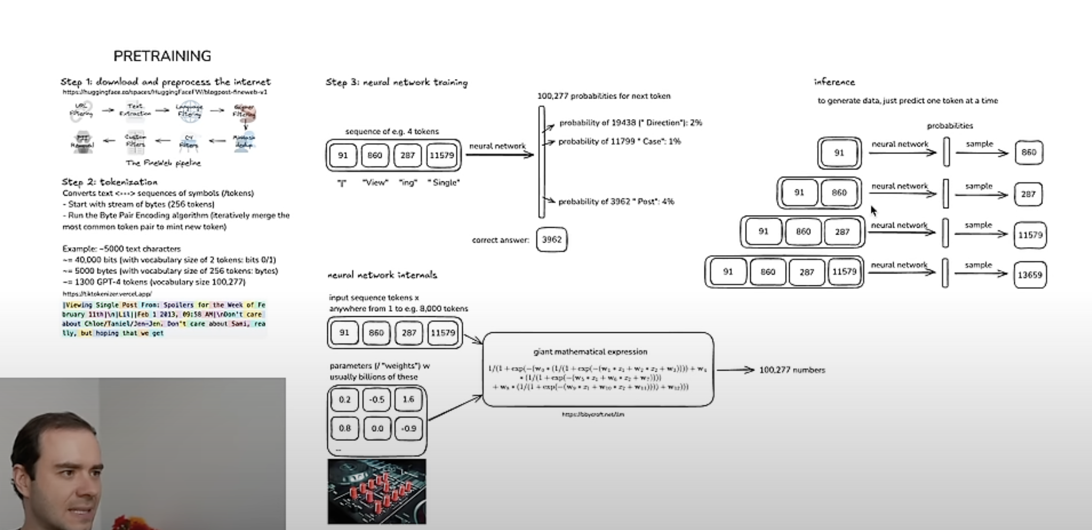
Stage 1: Pre-Training
Step 1 — Download and process the internet
Raw web data goes through a pipeline (e.g. FineWeb): URL filters (CommonCrawl) → text extraction → quality filters. This produces the pre-training dataset.
Step 2 — Tokenization
NNs expect a 1D sequence of symbols from a finite vocabulary. Raw text is compressed using the byte pair encoding (BPE) algorithm: repeatedly merge the most frequent adjacent symbol pair into a new token. The result is a vocabulary. Play with GPT-4 tokenization at tiktokenizer.vercel.app.
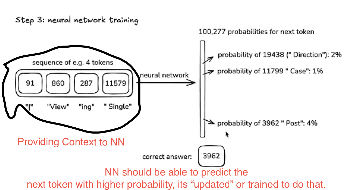
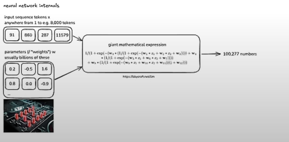
Step 3 — Training the Neural Network
The NN (a transformer) is a giant mathematical expression. Training adjusts its parameters so the probability of the next token matches the training distribution.
Visualize internals at bbycroft.net/llm.
Step 4 — Inference
Generating new tokens from the trained model. ChatGPT only does the inference part (plus the assistant layer on top). Pre-training and tokenization happen once; inference runs on every query.
The Base Model
A base model is an internet document simulator — given prefix tokens, it predicts the next token based on everything it saw during training. It is stochastic by nature.
- Information seen more often in training → remembered more reliably
- Regurgitation: reciting training data verbatim (undesirable)
- Hallucination: best-guess token prediction when the model hasn’t seen the answer
Base models are not assistants. They are glorified autocomplete. Few-shot prompting is a trick to coax assistant-like behavior from a base model.
Released base models need two things: the Python code (e.g. openai/gpt-2) and the parameter weights (just numbers). Play with open base models at app.hyperbolic.xyz.
Stage 2: Post-Training — Making an Assistant
All the heavy compute/data/cost is in pre-training. Post-training is relatively cheap and fast.
- Humans write a dataset of conversations (question + ideal answer pairs)
- Conversations are tokenized (similar protocol to pre-training)
- Base model is fine-tuned on this data → Supervised Fine-Tuning (SFT)
This is called the InstructGPT paper approach. OpenAI didn’t release the data; HuggingFace OpenAssistant is an OSS equivalent.
The model now has a “human labeler persona” — it answers questions in the style of the experts who wrote the training conversations. If the prompt matches the post-training distribution, the SFT model responds. Otherwise it falls back to pre-training knowledge (the whole internet).
Today, LLMs themselves are used to generate post-training data (e.g. UltraChat), eliminating the need for humans.
LLM Physiology
Hallucinations
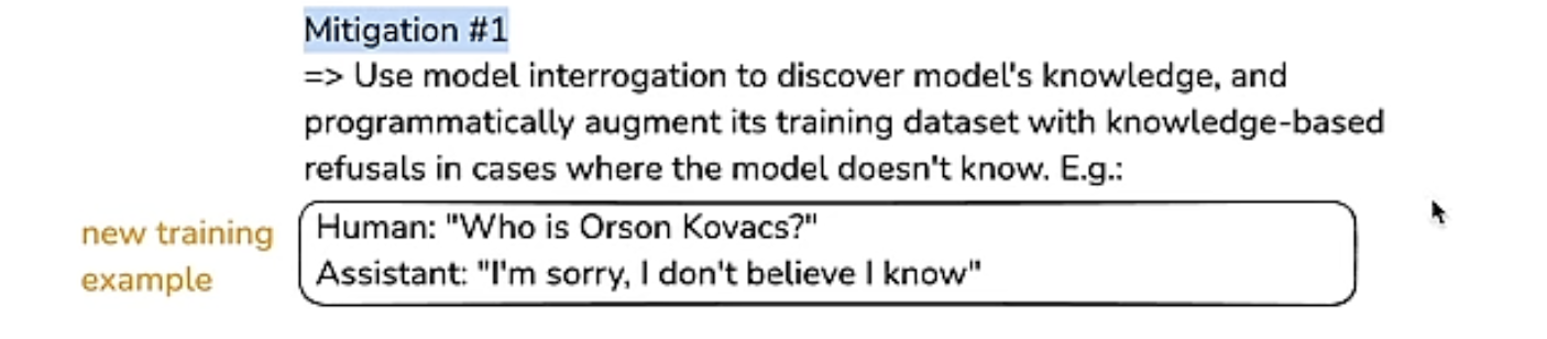
The model statistically emits tokens from its training distribution. For questions it doesn’t know the answer to, it confidently guesses. Mitigations:
- Teach uncertainty: train the model on examples where the answer is “I don’t know” so the relevant neurons activate on uncertainty (ref)
- External tools: model detects uncertainty, emits a special
<SEARCH_WEB>token, fetches new data, adds it to the context window, then infers from the richer context. Knowledge in model parameters = vague recollection; knowledge in context window tokens = working memory.
Knowledge of Self
Without intervention, a model asked “Who are you?” gives a statistically plausible answer (often “ChatGPT by OpenAI”) because that text is prevalent in pre-training data — even if the model is something else entirely. Fix: hardcode a system prompt at conversation start, or fine-tune with identity-specific conversations.
Models Need Time to Think
Each token spends a finite amount of compute in the NN. To solve hard problems:
- Spread computation across tokens — let the model “think out loud” before answering
- Use a code interpreter — models can’t do mental arithmetic but can write and run Python
- Models are bad at spelling because they see tokens (chunks), not individual characters; the tokenizer isn’t character-aware
Summary: Three Stages
| Stage | What it does | Training data |
|---|---|---|
| Pre-training | Internet document simulator | The entire internet |
| Post-training (SFT) | Assistant with human persona | Human-written Q&A conversations |
| RLFT | Reasoning / “thinking” models | Verifiable Q&A + trial-and-error |
RLFT (Reinforcement Learning on Fine-Tuned models): generate many candidate answers, pick the best, train on it, repeat. All major providers do this internally; DeepSeek was the first to open-source the approach and demonstrate its “reasoning” capability. Models learn to allocate more tokens to thinking — essentially chain-of-thought emerging from RL.
GPT-o*series = thinking/reasoning models (RLFT)GPT-4*series = mostly SFT post-trained models- For factual questions → SFT models. For math/logic → reasoning models.
RLHF (Reinforcement Learning from Human Feedback): extends RL to unverifiable domains by training a “reward model” NN on human preferences, then using it as a simulator. Downside: the reward function can be gamed since it’s a NN approximation, not real human feedback.
Future Capabilities
- Multimodal: audio, video, images are just more tokens — same model handles all modalities
- Agents: models operating autonomously over longer horizons
- Test-time training: currently impossible to add knowledge after training except via the (finite) context window; multimodal use cases will push context windows larger
How to Keep Up
- lmarena.ai — human-preference model rankings (somewhat gamed, but good first pass)
- ainews newsletter — daily summaries
How to Access Models
| Type | Where |
|---|---|
| Proprietary (GPT, Gemini) | chatgpt.com, gemini.google.com |
| Open-weight (DeepSeek, LLaMA) | together.ai |
| Base models | hyperbolic.xyz |
| Run locally | LM Studio |